Steps1-6

Load the R packages we will use

library(tidyverse)
library(echarts4r)
library(hrbrthemes)

Read the data in the files, drug_cos.csv,health_cos.csvinto R and assign to the variable drug_cos and health_cos, respectively.

drug_cos <- read_csv("https://estanny.com/static/week6/drug_cos.csv")
health_cos <- read_csv("https://estanny.com/static/week6/health_cos.csv")

Use glimpse to get a glimpse of the data.

drug_cos %>% glimpse()

Rows: 104
Columns: 9
$ ticker       <chr> "ZTS", "ZTS", "ZTS", "ZTS", "ZTS", "ZTS", "ZTS…
$ name         <chr> "Zoetis Inc", "Zoetis Inc", "Zoetis Inc", "Zoe…
$ location     <chr> "New Jersey; U.S.A", "New Jersey; U.S.A", "New…
$ ebitdamargin <dbl> 0.149, 0.217, 0.222, 0.238, 0.182, 0.335, 0.36…
$ grossmargin  <dbl> 0.610, 0.640, 0.634, 0.641, 0.635, 0.659, 0.66…
$ netmargin    <dbl> 0.058, 0.101, 0.111, 0.122, 0.071, 0.168, 0.16…
$ ros          <dbl> 0.101, 0.171, 0.176, 0.195, 0.140, 0.286, 0.32…
$ roe          <dbl> 0.069, 0.113, 0.612, 0.465, 0.285, 0.587, 0.48…
$ year         <dbl> 2011, 2012, 2013, 2014, 2015, 2016, 2017, 2018…

health_cos %>% glimpse()

Rows: 464
Columns: 11
$ ticker      <chr> "ZTS", "ZTS", "ZTS", "ZTS", "ZTS", "ZTS", "ZTS"…
$ name        <chr> "Zoetis Inc", "Zoetis Inc", "Zoetis Inc", "Zoet…
$ revenue     <dbl> 4233000000, 4336000000, 4561000000, 4785000000,…
$ gp          <dbl> 2581000000, 2773000000, 2892000000, 3068000000,…
$ rnd         <dbl> 427000000, 409000000, 399000000, 396000000, 364…
$ netincome   <dbl> 245000000, 436000000, 504000000, 583000000, 339…
$ assets      <dbl> 5711000000, 6262000000, 6558000000, 6588000000,…
$ liabilities <dbl> 1975000000, 2221000000, 5596000000, 5251000000,…
$ marketcap   <dbl> NA, NA, 16345223371, 21572007994, 23860348635, …
$ year        <dbl> 2011, 2012, 2013, 2014, 2015, 2016, 2017, 2018,…
$ industry    <chr> "Drug Manufacturers - Specialty & Generic", "Dr…

Which variables are the same in both data sets

names_drugs <- drug_cos %>% names()
names_health <- health_cos %>% names()
intersect(names_drugs,names_health)

[1] "ticker" "name"   "year"

Select subset of variables to work with

For drug_cos select (in this order): ticker, year,grossmargin -Extract observations for 2018 -Assign output to drug_subset
For health_cos select (in this order): ticker,year,revenue,gp,industry
Extract observations for 2018
Assign output to health_subset

drug_subset <- drug_cos %>% 
  select(ticker,year,grossmargin) %>% 
  filter(year==2018)
health_subset <- health_cos %>% 
  select(ticker,year,revenue,gp,industry) %>% 
  filter(year==2018)

Keep all the rows and columns drug_subset join with columns health_subset

drug_subset%>% left_join(health_subset)

# A tibble: 13 x 6
   ticker  year grossmargin   revenue        gp industry              
   <chr>  <dbl>       <dbl>     <dbl>     <dbl> <chr>                 
 1 ZTS     2018       0.672   5.82e 9   3.91e 9 Drug Manufacturers - …
 2 PRGO    2018       0.387   4.73e 9   1.83e 9 Drug Manufacturers - …
 3 PFE     2018       0.79    5.36e10   4.24e10 Drug Manufacturers - …
 4 MYL     2018       0.35    1.14e10   4.00e 9 Drug Manufacturers - …
 5 MRK     2018       0.681   4.23e10   2.88e10 Drug Manufacturers - …
 6 LLY     2018       0.738   2.46e10   1.81e10 Drug Manufacturers - …
 7 JNJ     2018       0.668   8.16e10   5.45e10 Drug Manufacturers - …
 8 GILD    2018       0.781   2.21e10   1.73e10 Drug Manufacturers - …
 9 BMY     2018       0.71    2.26e10   1.60e10 Drug Manufacturers - …
10 BIIB    2018       0.865   1.35e10   1.16e10 Drug Manufacturers - …
11 AMGN    2018       0.827   2.37e10   1.96e10 Drug Manufacturers - …
12 AGN     2018       0.861   1.58e10   1.36e10 Drug Manufacturers - …
13 ABBV    2018       0.764   3.28e10   2.50e10 Drug Manufacturers - …

Qestion join_ticker

Start with drug_cos
Extract observations for the ticker JNJ from drug_cos
Assign output to the variable drug_cos_subset

drug_cos_subset <- drug_cos %>%
  filter(ticker=="JNJ")

Display drug_cos_subset

drug_cos_subset

# A tibble: 8 x 9
  ticker name  location ebitdamargin grossmargin netmargin   ros   roe
  <chr>  <chr> <chr>           <dbl>       <dbl>     <dbl> <dbl> <dbl>
1 JNJ    John… New Jer…        0.247       0.687     0.149 0.199 0.161
2 JNJ    John… New Jer…        0.272       0.678     0.161 0.218 0.173
3 JNJ    John… New Jer…        0.281       0.687     0.194 0.224 0.197
4 JNJ    John… New Jer…        0.336       0.694     0.22  0.284 0.217
5 JNJ    John… New Jer…        0.335       0.693     0.22  0.282 0.219
6 JNJ    John… New Jer…        0.338       0.697     0.23  0.286 0.229
7 JNJ    John… New Jer…        0.317       0.667     0.017 0.243 0.019
8 JNJ    John… New Jer…        0.318       0.668     0.188 0.233 0.244
# … with 1 more variable: year <dbl>

Use left_join to combine the rows and columns of drug_cos_subset with the columns of health_cos

combo_df <- drug_cos_subset %>%
  left_join(health_cos)

Display combo_df

combo_df

# A tibble: 8 x 17
  ticker name  location ebitdamargin grossmargin netmargin   ros   roe
  <chr>  <chr> <chr>           <dbl>       <dbl>     <dbl> <dbl> <dbl>
1 JNJ    John… New Jer…        0.247       0.687     0.149 0.199 0.161
2 JNJ    John… New Jer…        0.272       0.678     0.161 0.218 0.173
3 JNJ    John… New Jer…        0.281       0.687     0.194 0.224 0.197
4 JNJ    John… New Jer…        0.336       0.694     0.22  0.284 0.217
5 JNJ    John… New Jer…        0.335       0.693     0.22  0.282 0.219
6 JNJ    John… New Jer…        0.338       0.697     0.23  0.286 0.229
7 JNJ    John… New Jer…        0.317       0.667     0.017 0.243 0.019
8 JNJ    John… New Jer…        0.318       0.668     0.188 0.233 0.244
# … with 9 more variables: year <dbl>, revenue <dbl>, gp <dbl>,
#   rnd <dbl>, netincome <dbl>, assets <dbl>, liabilities <dbl>,
#   marketcap <dbl>, industry <chr>

Note the variables ticker.name,location and industry are the same for all observations.
Assign the company name to co_name

co_name <- combo_df %>%
  distinct(name) %>% 
  pull()

Assign the company location to co_location

co_location <- combo_df %>%
  distinct(location) %>% 
  pull()

Assign the company location to co_industry

co_industry <- combo_df %>%
  distinct(industry) %>% 
  pull()

Put the r inline commands used in the blanks below. When you knit the document the results of the commands will be displayed in your text. The company Answer is located in Answer and is a member of the Answer industry group.

The company Johnson & Johnson is located in New Jersey; U.S.A and is a member of Drug Manufacturers - General industry group.

Start with combo_df
Select variables (in this order): year, grossmargin, netmargin, revenue, gp, net income Assign the output to combo_df_subset

combo_df_subset <- combo_df %>% 
  select(year, grossmargin, netmargin, revenue, gp, netincome)

Display combo_df_subset

 combo_df_subset

# A tibble: 8 x 6
   year grossmargin netmargin     revenue          gp   netincome
  <dbl>       <dbl>     <dbl>       <dbl>       <dbl>       <dbl>
1  2011       0.687     0.149 65030000000 44670000000  9672000000
2  2012       0.678     0.161 67224000000 45566000000 10853000000
3  2013       0.687     0.194 71312000000 48970000000 13831000000
4  2014       0.694     0.22  74331000000 51585000000 16323000000
5  2015       0.693     0.22  70074000000 48538000000 15409000000
6  2016       0.697     0.23  71890000000 50101000000 16540000000
7  2017       0.667     0.017 76450000000 51011000000  1300000000
8  2018       0.668     0.188 81581000000 54490000000 15297000000

Create the variable grossmargin_check to compare with the variable grossmargin. They should be equal. grossmargin_check = gp / revenue Create the variable close_enough to check that the absolute value of the difference between grossmargin_check and grossmargin is less than 0.001

combo_df_subset %>% 
  mutate(grossmargin_check=gp/revenue, close_enough=abs(grossmargin_check - grossmargin) < 0.001)

# A tibble: 8 x 8
   year grossmargin netmargin revenue      gp netincome
  <dbl>       <dbl>     <dbl>   <dbl>   <dbl>     <dbl>
1  2011       0.687     0.149 6.50e10 4.47e10   9.67e 9
2  2012       0.678     0.161 6.72e10 4.56e10   1.09e10
3  2013       0.687     0.194 7.13e10 4.90e10   1.38e10
4  2014       0.694     0.22  7.43e10 5.16e10   1.63e10
5  2015       0.693     0.22  7.01e10 4.85e10   1.54e10
6  2016       0.697     0.23  7.19e10 5.01e10   1.65e10
7  2017       0.667     0.017 7.64e10 5.10e10   1.30e 9
8  2018       0.668     0.188 8.16e10 5.45e10   1.53e10
# … with 2 more variables: grossmargin_check <dbl>,
#   close_enough <lgl>

Create the variable netmargin_check to compare with the variable netmargin. They should be equal. -Create the variable close_enough to check that the absolute value of the difference between netmargin_check and netmargin is less than 0.001

 combo_df_subset %>% 
   mutate(netmargin_check = netincome/revenue,
  close_enough =  abs(netmargin_check - netmargin) < 0.001)

# A tibble: 8 x 8
   year grossmargin netmargin revenue      gp netincome
  <dbl>       <dbl>     <dbl>   <dbl>   <dbl>     <dbl>
1  2011       0.687     0.149 6.50e10 4.47e10   9.67e 9
2  2012       0.678     0.161 6.72e10 4.56e10   1.09e10
3  2013       0.687     0.194 7.13e10 4.90e10   1.38e10
4  2014       0.694     0.22  7.43e10 5.16e10   1.63e10
5  2015       0.693     0.22  7.01e10 4.85e10   1.54e10
6  2016       0.697     0.23  7.19e10 5.01e10   1.65e10
7  2017       0.667     0.017 7.64e10 5.10e10   1.30e 9
8  2018       0.668     0.188 8.16e10 5.45e10   1.53e10
# … with 2 more variables: netmargin_check <dbl>, close_enough <lgl>

Question Sumarize_Industry

Fill in the blanks Put the command you use in the Rchunks in the Rmd file for this quiz -Use the health_cos data
For each industry calculate
mean_netmargin_percent = mean(netincome / revenue) * 100
median_netmargin_percent = median(netincome / revenue) * 100
min_netmargin_percent = min(netincome / revenue) * 100
max_netmargin_percent = max(netincome / revenue) * 100

health_cos  %>% 
  group_by(industry)  %>% 
  summarize(mean_netmargin_percent =mean( netincome /revenue ) * 100,
          median_netmargin_percent =  median( netincome / revenue) * 100,
             min_netmargin_percent =  min( netincome / revenue) * 100,
             max_netmargin_percent =  max( netincome / revenue) * 100) %>% 
  knitr::kable()

industry	mean_netmargin_percent	median_netmargin_percent	min_netmargin_percent	max_netmargin_percent
Biotechnology	-4.657436	7.621995	-197.4908687	68.804898
Diagnostics & Research	13.139154	12.332078	0.3990080	26.344477
Drug Manufacturers - General	19.358281	19.537586	-34.8658185	100.853774
Drug Manufacturers - Specialty & Generic	5.879275	9.008114	-75.9913646	24.515021
Healthcare Plans	3.283594	3.374305	-0.3052745	6.020507
Medical Care Facilities	6.101918	6.458909	1.3975983	8.304696
Medical Devices	12.363459	14.284582	-56.1180853	49.362818
Medical Distribution	1.700144	1.033174	-0.1016205	4.513858
Medical Instruments & Supplies	12.313479	13.978242	-47.0569354	48.853685

-mean_netmargin_percent for the industry Medical Care Facilities is -median_netmargin_percent for the industry Medical Care Facilities is -min_netmargin_percent for the industry Medical Care Facilities is -max_netmargin_percent for the industry Medical Care Facilities is

Question inline_ticker

Fill in the blanks
Use the health_cos data
Extract observations for the ticker ZTS from health_cos and assign to the variable health_cos_subset

health_cos_subset  <- health_cos  %>% 
   filter(ticker == "ZTS")

Display health_cos_subset health_cos_subset

health_cos_subset

# A tibble: 8 x 11
  ticker name  revenue     gp    rnd netincome  assets liabilities
  <chr>  <chr>   <dbl>  <dbl>  <dbl>     <dbl>   <dbl>       <dbl>
1 ZTS    Zoet…  4.23e9 2.58e9 4.27e8    2.45e8 5.71e 9  1975000000
2 ZTS    Zoet…  4.34e9 2.77e9 4.09e8    4.36e8 6.26e 9  2221000000
3 ZTS    Zoet…  4.56e9 2.89e9 3.99e8    5.04e8 6.56e 9  5596000000
4 ZTS    Zoet…  4.78e9 3.07e9 3.96e8    5.83e8 6.59e 9  5251000000
5 ZTS    Zoet…  4.76e9 3.03e9 3.64e8    3.39e8 7.91e 9  6822000000
6 ZTS    Zoet…  4.89e9 3.22e9 3.76e8    8.21e8 7.65e 9  6150000000
7 ZTS    Zoet…  5.31e9 3.53e9 3.82e8    8.64e8 8.59e 9  6800000000
8 ZTS    Zoet…  5.82e9 3.91e9 4.32e8    1.43e9 1.08e10  8592000000
# … with 3 more variables: marketcap <dbl>, year <dbl>,
#   industry <chr>

In the console, type ?distinct. Go to the help pane to see what distinct does
In the console, type ?pull. Go to the help pane to see what pull does
Run the code below

health_cos_subset  %>% 
  distinct(name) %>%  
  pull(name)

[1] "Zoetis Inc"

Assign the output to co_name

 co_name <- health_cos_subset  %>% 
  distinct(name) %>% 
  pull(name)

You can take output from your code and include it in your text.

The name of the company with ticker ZTS is Zoetis Inc In following chuck
Assign the company’s industry group to the variable co_industry

co_industry  <- health_cos_subset  %>% 
   distinct(industry) %>% 
   pull()

This is outside the Rchunck. Put the r inline commands used in the blanks below. When you knit the document the results of the commands will be displayed in your text.

The company Zoetis Inc is a member of the Drug Manufacturers - Specialty & Generic group.

Steps 7-11

Prepare the data for the plots

start with health_cos THEN
group_by industry THEN
calculate the median research and development expenditure by industry assign the output to df

df <- health_cos %>%
  group_by(industry) %>% 
  summarize(med_rnd_rev = median(rnd/revenue))

Use glimpse to glimpse the data for the plots

df %>% glimpse()

Rows: 9
Columns: 2
$ industry    <chr> "Biotechnology", "Diagnostics & Research", "Dru…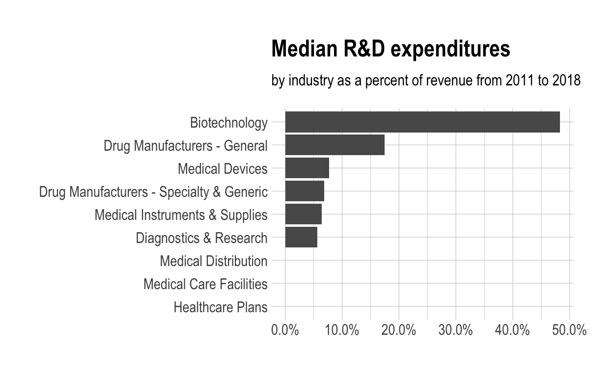
$ med_rnd_rev <dbl> 0.48317287, 0.05620271, 0.17451442, 0.06851879,…

Create a static bar chart

Use ggplot to initialize the chart
data is df
the variable industry is mapped to the x-axis
- reorder is based the value of med_rnd_rev
the variable med_rnd_rev is mapped in the y-axis
add a bar chart using geom_col
use scale_y_continuous to label the y-axis with percent
use coord_flip() to flip the coordinates
use labs to add title, subtitle and remove x and y-axes
use theme_ipsum()from the hrbrthemes package to imporve the theme

ggplot(data = df, mapping = aes(
  x = reorder(industry, med_rnd_rev ),
  y = med_rnd_rev
  ))+
  geom_col()+
  scale_y_continuous(labels= scales::percent)+
  coord_flip()+
  labs(
    title= "Median R&D expenditures",
    subtitle= "by industry as a percent of revenue from 2011 to 2018",
    x=NULL,y=NULL)+
  theme_ipsum()

Save the last plot to preview.png and add to the yaml chunk at the top

ggsave(filename="preview.png", 
   path = here::here("_posts","2021-03-13-joining-data"))

Joining data

Steps1-6

Qestion join_ticker

Question Sumarize_Industry

Question inline_ticker

Steps 7-11